The Transformer as a Differentiable Computer

Summary

The transformer neural network was invented in 2017 by the Google Brain team1. This architecture finds applications across various domains in deep learning, ranging from large language models such as ChatGPT to cutting-edge image generation methods like Stable Diffusion2. Understanding the architecture is therefore crucial. Its remarkable ability to generalize can be attributed to its fundamental nature as a differentiable computer. In this essay, we will explore how this connection can be established. In the end, we will take a short look at my implementation of the architecture and test it by generating tiny stories. You can find my implementation here3.

What is a computer?

Generally, a computer can be understood as a machine that receives input and computes an output based on a predefined algorithm. Moreover, the famous Turing machine operates on a tape, serving as the memory component of the algorithm. Fundamentally, a Turing machine possesses the following three capabilities:

1. With a tape head, the Turing machine can read from or write to the tape.
2. The head can move to different positions.
3. The movements and writing operations occur in an intelligent manner (transition function).

We will see how the transformer architecture implements versions of all these capabilities. More precisely, the first two capabilities are implemented by the so-called attention mechanism.

The attention mechanism

The tape of the transformer is given as a list of so-called embedding vectors. An embedding vector describes a token from the tape and is just a list of numbers. The length of this vector, d_k, is specified before training the transformer. The longer the vector, the more information it can store. The tape looks like this:

In the above example we chose d_k = 3, so each token is represented by three numbers. Note that the tape has finite length, in contrast to the Turing machine.

Reading from the tape

We now want the tokens to communicate with each other—for example, to read and write from the tape. However, because we want to optimize the computer with gradient-descent techniques, this operation has to be differentiable. To achieve this, each token t generates three pieces of information:

• Query(t): What type of information am I seeking?
• Key(t): What type of information do I represent?
• Value(t): What actual information do I contain?

To calculate these values, we use a simple feed-forward network: one linear projection. This projection will later be learned by the neural network, and all tokens use the same linear projections. We define linear projections q, k, v ∈ ℝ^{d_k × d_k} and then Query(t_i) = t_iq for every token t_i. Similarly, Key(t_i) = t_ik and Value(t_i) = t_iv.

Each token t now takes its own query information and compares it with the key information of every other token. That way, t can find the token t′ whose information best matches its query and copy Value(t′) onto the tape. The comparison can be implemented as any function that calculates the similarity of two vectors: if the query of one token is very similar to the key of another, the score should be high.

In practice this is often done using the dot product, because it can be calculated very efficiently. In essence, the dot product calculates the length of the projection of one vector onto another (if normalized). If two vectors point in the same direction, the score is very high. If they are orthogonal, the score is zero.

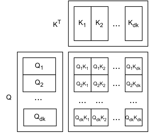
This is even more powerful than the original Turing machine, as we can copy tokens from anywhere on the tape. Furthermore, we do this in a much more dynamic way: tokens can search for specific information due to the query/key structure. All of this is done for every token in parallel. But how can we calculate it efficiently? Let T ∈ ℝ^{t × d_k} be our tape, where t is the number of tokens. Let Q = Tq, K = Tk, and V = Tv be the generated queries, keys, and values. Then

QK^T

calculates the dot product of every query with every key in parallel. Entry (i, j) of this matrix tells us how much token t_i wants the information of token t_j.

To copy the desired information to the tape, we can do the following:

A = (QK^T)V

If each row of QK^T contains exactly one element with a value of one, each token copies exactly one of the other tokens to the tape:

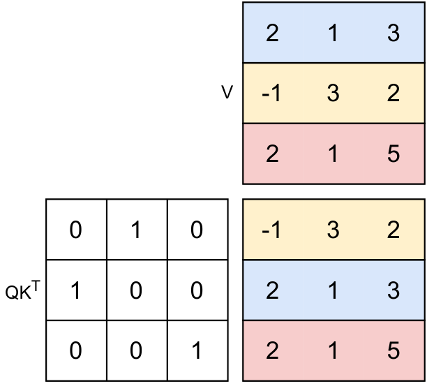
However, because the rows of QK^T are not necessarily normalized to a probability distribution and can take on very large values, the information would accumulate. To prevent this, we convert each row to a probability distribution: entry (i, j) should tell us how much of token j’s information token i wants. For example, if entry (i, j) is 0.6, it will contain 60 percent of the value of token j.

One way to do this is to divide every entry by the sum of its row. The softmax function used in the original paper does exactly that, except that it exponentiates the values first. Exponentiation amplifies the differences between values, allowing the network to focus on particular parts of the tape more effectively.

A = softmax(QK^T)V

To stabilize training, the QK^T matrix is scaled down by a factor of √d_k. This keeps the variance of the distribution at one (if it was one before). The main reason for doing this is that the softmax function has very small gradients when its input values are large, making it difficult for gradient descent to improve the network. The authors of “Attention Is All You Need”1 show that this normalization factor improves the performance of the attention mechanism. The final attention mechanism is therefore:

A = softmax(QK^T / √d_k)V

Positional embedding

One problem remains: this communication mechanism is completely position-independent. The tokens do not know where they are or from which position they read. The tape is treated as a bag of tokens instead of an array of tokens. Looking again at the dot-product figure, each token compares its query with the keys of every other token, and the resulting matrix is used to extract information. Shuffling the tape beforehand does not change how much one token attends to the others.

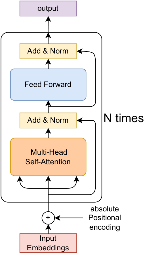
We cannot ignore the positions of tokens because they matter for many algorithms, such as sorting. One solution is to add positional information to the tokens themselves: every token additionally stores its own position. This can be done by learning a positional embedding during training and overlaying it on the token embeddings. As we will see later, however, this is not always the most effective approach.

The transition function

We have seen how information can be exchanged on the tape. Now we want to use that information to calculate a new token and write it back to the tape. We map the accumulated information from the attention mechanism through a simple multilayer perceptron. This neural network maps to the output token we want to write. The “state” of the computer can be thought of as a section of the token embedding.

The Transformer

Combining the attention mechanism with the multilayer perceptron (MLP) simulates one step of the computer. To simulate multiple steps, we repeat these two components N times. The more blocks we connect in series, the more complicated the algorithms the transformer can calculate in theory.

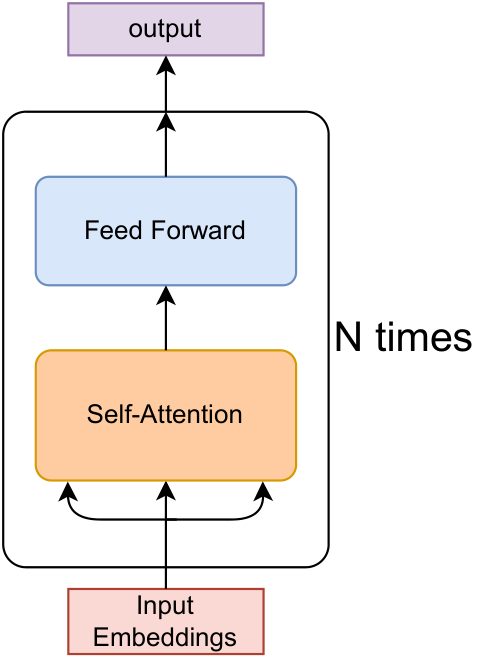
There are limitations in this architecture compared with a Turing machine. First, we can simulate only a constant number of steps. The tape also does not have infinite length. Nevertheless, this is enough for most algorithms because we have a much more powerful way to exchange information: all tokens communicate with one another and transition to their next values in parallel. In a sense, we perform many steps of computation in parallel, while a Turing machine can perform only one step at a time.

We can also store much more diverse information at each token, depending on the size of the embedding vector d_k. Embedding vectors can store all kinds of information, such as the position or the state of the computer at a token. These advantages outweigh the limitations and make the architecture an efficient differentiable computer.

The architecture outlined above is already powerful in theory, but there are several improvements that make it more effective in practice.

Skip connections

To train the network successfully, we introduce skip connections4. We add the values before the attention mechanism to the values after the attention mechanism, and do the same around the multilayer perceptron. This lets gradients flow back to the first layers, allowing the model to train effectively. Skip connections reduce the vanishing-gradient problem and allow the transformer to learn simple algorithms early in training and extend them into more complex algorithms later.

Batch normalization

Another way to improve training stability is to add normalization layers. These make sure that the mean of the data is zero and that its variance stays constant. This tends to make training more stable, although the reasons for its effectiveness are still an active topic of research.

Multi-headed attention

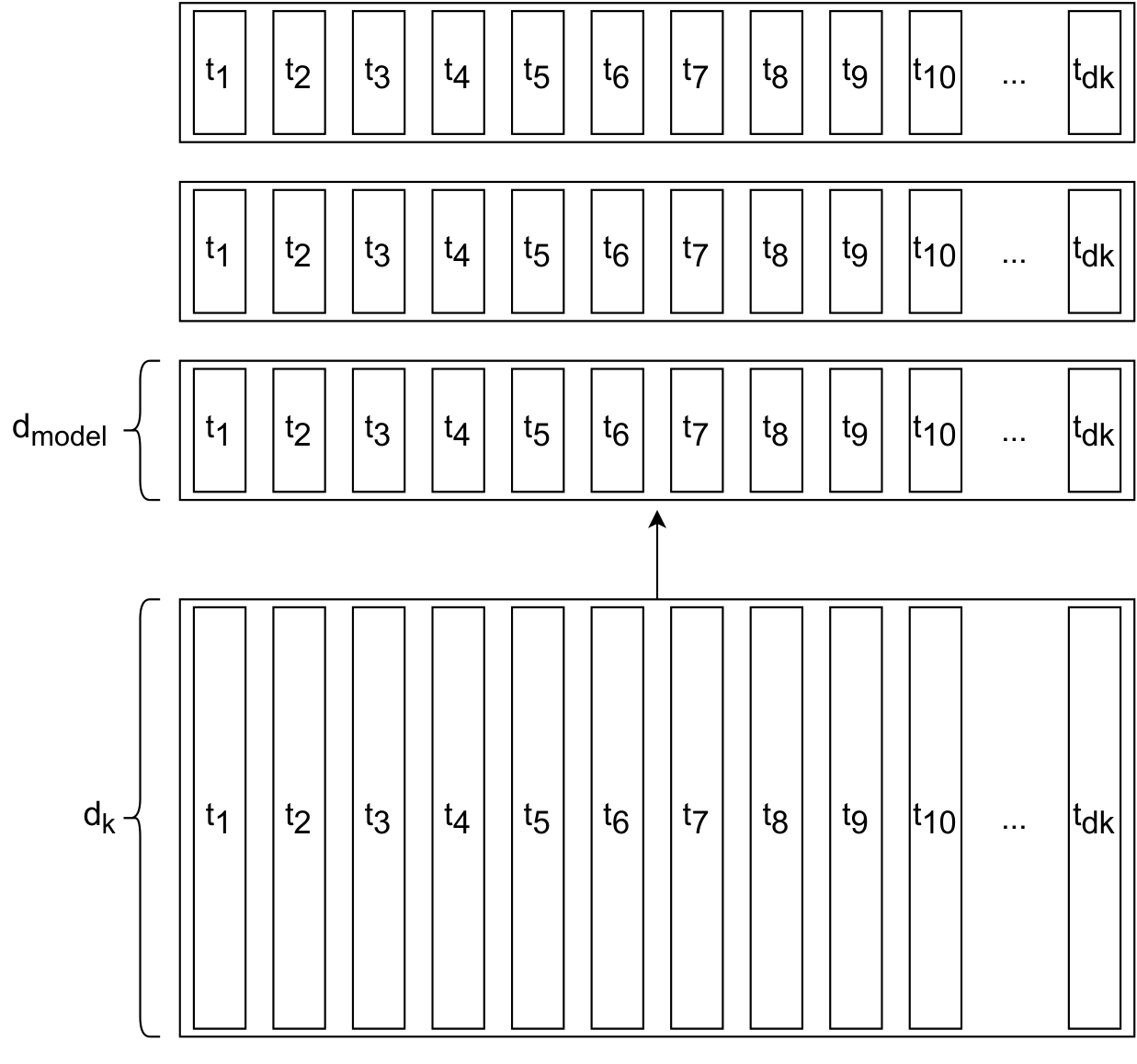
To make the architecture even more efficient, we can split the tape into multiple smaller tapes and perform communication on each of them in parallel. This is done by dividing the embedding vectors into chunks. In the figure below, the tape is split into three smaller tapes of length d_model, such that 3 · d_model = d_k. Attention is performed on each smaller tape before the results are merged back into one large tape. This enables a richer and more efficient exchange of information.

Modern adaptations

The architecture outlined earlier is already effective and has stayed largely the same over time. One weakness, however, is positional encoding. Positional information is stored directly inside the tokens and must therefore pass from layer to layer. Eventually it can be lost, leading to less efficient communication.

Almost all modern LLMs, such as Llama 25, use a different approach. Instead of storing positional information inside the tokens, they implement it directly in the attention mechanism by assigning lower attention scores to tokens that are far apart. Tokens thereby know where they are relative to each other.

The most popular approach is rotary positional embedding6, where tokens are rotated in the embedding space according to their position. Another simple but effective approach is Attention with Linear Biases (ALiBi)7. Here a bias is added to the attention scores so that distant tokens exchange less information:

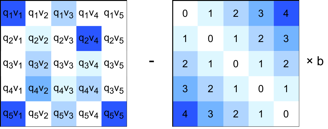
It is also possible to penalize each attention head differently by adjusting the value of b. In some heads, tokens can communicate only with nearby tokens; in others, every token may communicate with every other token. This lets the model capture positional information effectively. The ALiBi paper proposes decreasing b exponentially—for eight attention heads, using the values 2⁻¹, 2⁻², …, 2⁻⁸.

One disadvantage of this method is that we cannot use techniques such as FlashAttention8 without adapting how the bias is applied inside the attention mechanism. I still used ALiBi in my implementation because it is easy to implement.

Implementation

To test the transformer architecture, I trained it on a simple text dataset called TinyStories9. To generate text, we must adapt the architecture slightly. For efficient training, we feed in a training text and let the network predict the next token for every prefix of the sample. We shift the input text one position to the left and take the cross-entropy loss against the model output. The model output is converted to a probability distribution over all tokens.

Some attention weights must also be masked because tokens must not communicate with the future—otherwise predicting the next token would be trivial:

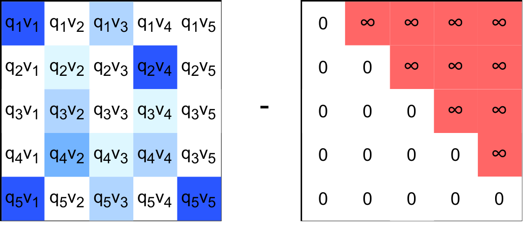
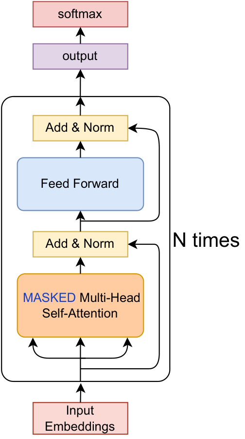
The mask is applied before the softmax function. Every disallowed entry therefore becomes zero while each row still sums to one. The final model is:

Architecture

I adopted the standard transformer architecture, except that I used ALiBi positional encoding as described above. I also moved the normalization layers in front of attention and the MLP. For weight initialization I used Xavier initialization, as proposed in this paper10. To reduce model size, I used weight tying for the input embedding and output projection. Everything is implemented in PyTorch.

I called the model “Alilama” because it uses ALiBi positional encoding and some techniques from the Llama 2 architecture. I tested the implementation with TinyStories, a dataset of simple stories generated by a capable language model. The clear structure and simplicity of the samples make it easy for a small model to learn basic language. Using this dataset, models with only two million parameters can generate grammatically correct English sentences.

Training

I used a simple training procedure: select random story fragments, combine them into batches, run them through the model, calculate cross-entropy loss, and update the model parameters with AdamW. There are many possible improvements, including warm-up iterations, gradient clipping, and cosine learning-rate decay as used by Llama 2. Since I wanted the implementation to remain simple, I omitted these features. I suspect the quality of the generations could be improved greatly by adding them.

Tokenization

Tokenization converts a string into a list of numbers, which is necessary because the model handles only numeric inputs. A simple approach is to use the bytes of the input string directly. This can be improved because some combinations of letters occur more frequently than others. Modern language models commonly use byte-pair encoding.

Byte-pair encoding starts with a training text converted into a byte sequence. It repeatedly selects the most frequent adjacent pair and merges it into a new token. The learned merges are stored in a dictionary. A new text is tokenized by applying those merges in the same order as during training. For TinyStories, I was able to compress the input to around 22 percent of its original size.

To train the tokenizer in a reasonable time, I made several low-level optimizations. The training algorithm uses a linked list for the input and tracks frequent pairs with a heap, as discussed in this paper11. The paper analyzes the algorithm as O(n log m), where n is the input size and m the vocabulary size. I suspect its running time is closer to O(n + m log m), which is effectively linear in practice, because the heap keys are changed only by one at a time. Implemented in C++, it could train on 100 MB of text in about a minute.

To speed up tokenization itself, I split text into chunks using regular expressions, a technique also used by tokenizers such as tiktoken12. With a multithreaded C++ implementation, I could tokenize 1 GB of text in around a minute. I called the implementation from Python through ctypes and used a byte-pair encoding framework13 created by Andrej Karpathy. The optimized implementation has not yet been added to that repository. You can also see my implementation here.

Results

I trained a model with only two million parameters: d_k = 128, eight transformer blocks, eight attention heads, an MLP hidden size of 512, and a context window of 128 tokens. I trained it for around four epochs, meaning the model saw the entire dataset four times. A larger model would obviously produce better results, but training resources were limited. Here are some completions; generated continuations are highlighted.

Once upon a time, Tom and Lisa found a shiny red apple. They both wanted it. Tom said, “I found it first!” Lisa said, “I want it too!” Tom said, “No, it’s mine!” They both pulled and pulled, but the apple did not move. Tom and Lisa were sad. They could not play with the apple anymore. They had to find a way to make the apple disappear. They could not agree on what to do. Then, Tom had an idea. He said, “Let’s share the apple!” They both agreed. They shared the apple and played together. They were happy and became friends.

When a ball is thrown into the air, it will eventually come back down.

Once upon a time there was a pumpkin. It was a very special pumpkin; it could speak. It was sad because it couldn’t move. Every day, it would say “hello” to the pumpkin. One day, a little girl named Lily saw the pumpkin. She wanted to be friends with it. She asked the pumpkin, “Can I be your friend?” The pumpkin said, “Yes, you can be my friend.” Lily was very happy. She played with the pumpkin all day. They had so much fun. But then, something unexpected happened. The pumpkin started to move! It was not a pumpkin at all! It was a magic pumpkin! The pumpkin said, “Thank you for the magic pumpkin. I was a magic pumpkin. Now, I can talk to you!” The pumpkin was very surprised. Lily and the pumpkin became best friends. They played together every day. The pumpkin was not sad anymore.

Once upon a time, there lived a black cat. The cat belonged to a little girl called Katie. Every day, Katie would take her cat for a walk in the park. One day, as Katie and her cat were walking around, they saw a mean-looking man. He said he wanted to take the cat, to which she replied, “This cat belongs to me.” Katie was sad, but she knew she had to be honest. She said, “I’m sorry, I didn’t know you were there.” The black cat was surprised but happy. She said, “It’s okay, I’m just happy to see you.” From that day on, Katie and her furry cat were best friends. They would often play together and have fun.

References

1. Ashish Vaswani, Noam Shazeer, Niki Parmar, Jakob Uszkoreit, Llion Jones, Aidan N. Gomez, Lukasz Kaiser, and Illia Polosukhin. “Attention Is All You Need.” (2017) arxiv.org/abs/1706.03762
2. Robin Rombach, Andreas Blattmann, Dominik Lorenz, Patrick Esser, and Björn Ommer. “High-Resolution Image Synthesis with Latent Diffusion Models.” arxiv.org/pdf/2112.10752.pdf
3. Johannes Voderholzer. “Training a Small GPT.” github.com/JohannesVod/Alilama
4. Kaiming He, Xiangyu Zhang, Shaoqing Ren, and Jian Sun. “Deep Residual Learning for Image Recognition.” arxiv.org/abs/1512.03385
5. Hugo Touvron et al. “Llama 2: Open Foundation and Fine-Tuned Chat Models.” (2023) arxiv.org/abs/2307.09288
6. Jianlin Su, Yu Lu, Shengfeng Pan, Ahmed Murtadha, Bo Wen, and Yunfeng Liu. “RoFormer: Enhanced Transformer with Rotary Position Embedding.” (2021) arxiv.org/abs/2104.09864
7. Ofir Press, Noah A. Smith, and Mike Lewis. “Train Short, Test Long: Attention with Linear Biases Enables Input Length Extrapolation.” arxiv.org/abs/2108.12409
8. Tri Dao. “FlashAttention-2: Faster Attention with Better Parallelism and Work Partitioning.” arxiv.org/abs/2307.08691
9. Ronen Eldan and Yuanzhi Li. “TinyStories: How Small Can Language Models Be and Still Speak Coherent English?” arxiv.org/abs/2305.07759
10. Xiao Shi Huang, Felipe Perez, Jimmy Ba, and Maksims Volkovs. “Improving Transformer Optimization Through Better Initialization.” cs.toronto.edu/~mvolkovs/ICML2020_tfixup.pdf
11. Vilém Zouhar, Clara Meister, Juan Luis Gastaldi, Li Du, Tim Vieira, Mrinmaya Sachan, and Ryan Cotterell. “A Formal Perspective on Byte-Pair Encoding.” paper PDF
12. OpenAI. “tiktoken.” github.com/openai/tiktoken
13. Andrej Karpathy. “minbpe.” github.com/karpathy/minbpe